Ori Finder. Part 1: Introduction

Welcome to a brand new REBELSCIENCE series called Ori Finder!

If you have followed our REBELSCIENCE lessons, you may already know our two companion series. DNA Toolkit is a beginner-friendly introduction to biology and Python. Genome Toolkit takes a closer look at the computer science and software engineering behind reliable bioinformatics tools. You can start Ori Finder here; we will recall the ideas we need as we go. In Genome Toolkit Part 2, we wrote count_kmer() to count a particular pattern in DNA. In Part 3, we added find_most_frequent_kmers() to find the patterns that occur most often. This time, we’ll use those familiar functions with a real chromosome and choose a new question for Ori Finder.

In This Part

We’ll begin with two Python functions we already know. Then we’ll get to know a few tiny friends: single-celled microorganisms called archaea. They will stay with us throughout Ori Finder, and may return in other series as our questions grow. We’ll start with one of them, see what questions we can ask with its DNA, and choose one: where does DNA copying begin? We’ll look at a small region that scientists have already studied, see what our counting functions tell us about its DNA patterns, and ask how we could search without knowing that region in advance.

Two Functions, Two Different Questions

Before we meet the organism we will study and the tool we will build, let’s briefly refresh how our two Genome Toolkit algorithms work. They will also be our first tools in Ori Finder, so it helps to see what each one can tell us. Let’s use one small DNA sequence: AAAGAAAATTGA. A k-mer is a short pattern of DNA letters. The k tells us how many letters are in it: AA is a 2-mer.

As we learned in Genome Toolkit, a small counting algorithm can answer a very specific question. count_kmer() answers the question “How many times does AA appear in this DNA?” We give the function two things: the sequence AAAGAAAATTGA and the exact pattern AA. It checks each possible starting place, moving forward one letter at a time. The first AAA contains two overlapping matches of AA; the later AAAA contains three. That makes 5 matches in total.

find_most_frequent_kmers() answers “Which 2-letter patterns appear most often?” We give it the same DNA, but this time we provide the length 2, not a particular pattern. It examines every 2-letter piece, counts the occurrences of each different pattern, and returns whichever pattern or patterns have the highest count. In this example, AA is the winner, with 5 occurrences. These two requests will help us turn a question about real DNA into something our Python program can examine.

Here’s what those two questions look like in Genome Toolkit. We put our small sequence into a DNA object, then ask each function for its answer.

small_dna = DNA(identifier="small_example", sequence="AAAGAAAATTGA")

count_result = count_kmer(small_dna, "AA")
# count_result.output.count = 5

frequent_result = find_most_frequent_kmers(small_dna, k_len=2)
# frequent_result.output.kmers = ["AA"]
# frequent_result.output.frequency = 5

Both calls happen to show the number 5, but they answer different questions. In the first, we choose the pattern and ask for its count. In the second, we choose a length and ask which pattern occurs most often. We can now use these two kinds of questions with real DNA.

Meet Pyrococcus abyssi

Now that we have refreshed our memory of those two simple bioinformatics algorithms, let’s meet the organism we will begin investigating. Even these small functions can reveal useful patterns in a complete genome. As our questions grow, we will add more algorithms, building a set of tools that helps us look more closely into the world of DNA. Our first organism is Pyrococcus abyssi, strain GE5. It’s a tiny archaeon that grows best at around 96°C / 205°F. Scientists first isolated it from a hot deep-sea environment in the North Fiji Basin, about 2,000 metres (6,600 feet) below the Pacific Ocean.

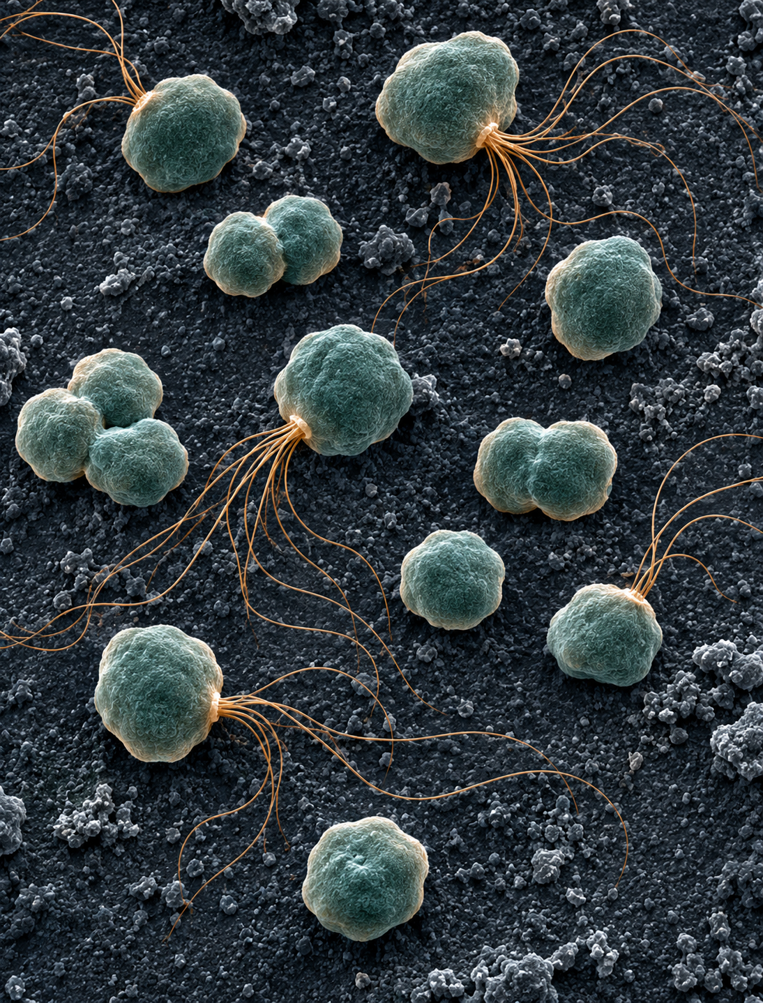
Deep underwater, hot mineral-rich water can flow out of the sea floor through places called hydrothermal vents. The pressure is enormous, and the microorganisms living there have adapted to conditions that would be far too hot for us.

Scientists have sequenced its complete chromosome, which contains 1,765,118 DNA bases. The National Center for Biotechnology Information (NCBI) provides that sequence in reference record NC_000868.1. An organism’s genome is its complete genetic information. For P. abyssi, this chromosome gives us the DNA sequence we’ll use in our first experiments.

One Genome, Five Questions

Our path begins with biology: a real organism and a question about its DNA. Its DNA sequence becomes data we can store in a FASTA file, and Python gives us tools to examine that data. This is where bioinformatics becomes interesting: we use computers to study biological data. Biology and chemistry help us interpret what we find; software engineering helps us build tools we can test and reuse. With just a few simple algorithms and a complete genome, we can already begin exploring our own research questions. There are many directions we could take. Here are just five:

1. Which DNA letters are most common? Count A, C, G and T, then compare the totals.
2. Which short DNA patterns repeat? Use our two familiar functions to find and count them.
3. Where are the genes? A gene is a section of DNA containing instructions used by a cell. We can explore the genes listed in the NCBI annotated record and investigate what researchers think they do.
4. How does this DNA compare with another organism’s DNA? Download a second genome and look for sequences that are alike or different.
5. Where does DNA copying begin? Can patterns in this long sequence help us find a likely starting area?

You can choose any of these questions, or use a genome from another organism that interests you. A brainstorming session with an LLM of your choice can help you think of possible research directions, then check its suggestions against real data and scientific sources. You can also follow the approach we take here: begin with a simple algorithm, explore a real genome, and notice which questions we can answer and what we are still missing. Understanding that gap helps us choose the next experiment or the next tool to build. That is how our investigation grows, one checked step at a time. For this new series, called Ori Finder, we will investigate question five.

Our Question: Where Does DNA Copying Begin?

Before a cell divides, it must make a copy of its chromosome. This process is called DNA replication. The copying begins in a region known as the origin of replication, or ori for short. Proteins help prepare this region, and DNA copying can then continue in two directions along the chromosome.

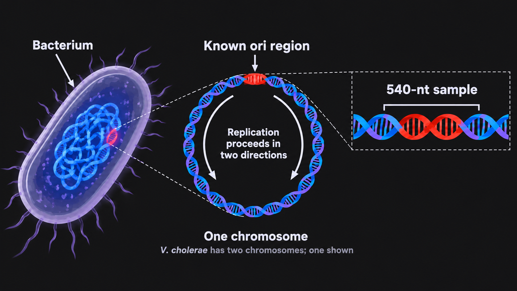
On the left of the illustration is a whole bacterium, Vibrio cholerae. In the middle is a circular DNA double helix illustrating one of its chromosomes, drawn separately so we can examine it. V. cholerae has two chromosomes; only one is shown here. On the right, we look more closely at a short stretch around the known starting region. The highlighted part of this circular chromosome shows where copying begins, and the arrows show the two directions. Our experiments use Pyrococcus, an archaeon, rather than this bacterium, but we can use the drawing to understand the question: how do we locate a small starting region in a long DNA sequence?

Researchers have already investigated the replication-origin area of P. abyssi. We can compare the DNA from that studied area with the patterns our functions find.

Our First Cheat: We Already Know Where to Look

The full chromosome has more than 1.7 million DNA letters. For our first look, we’ll use a much smaller piece that scientists have already studied. That gives us a familiar place to start before we search the entire chromosome.

We’ll get the DNA from NCBI reference NC_000868.1. NCBI lets us download the complete chromosome as a FASTA file: a text file with a short description at the top and the DNA letters underneath.

Scientists have already studied where copying begins in this organism. DoriC is a database that collects regions scientists describe as origins of replication, or likely origins, based on published research. It brings earlier scientific findings together so we have a place to look up a studied starting region instead of guessing where to begin. For P. abyssi, its historical record aORI10010003 points to a 799-letter region in this chromosome. So in this Part, we are not finding that location ourselves. We are taking it from earlier science and using it as a starting point for our own experiments. The DoriC 12.0 paper explains the database, and this earlier research paper explains how scientists studied the replication-origin area. NCBI supplies the complete chromosome, while DoriC points us toward the smaller research-annotated region. Together, these clues give us a manageable first example as we learn how to build and check our tool.

In Part 2, we’ll download the full chromosome and keep that FASTA file. Then we’ll copy the 799 letters from the known region into a second, smaller FASTA file. This is the known ori region from the same chromosome, not a different organism or an unrelated DNA sample. That way, we’ll have both the complete genome and the small piece we want to examine first. Later, the goal will be to work our way back toward this same region, and toward the short DNA patterns connected with the start of replication, without being handed the location first.

Our first clue is the location. Earlier research tells us which 799 letters to examine.

You don’t need to download anything or run code in this Part. The links are there if you want to explore the sources. We’ll download the DNA and try the Python functions ourselves in Part 2.

Our DNA sample

Organism: Pyrococcus abyssi GE5
Reference chromosome: NC_000868.1
Known teaching region: 799 DNA letters from historical DoriC record aORI10010003
Database context: DoriC 12.0 publication
File relationship: complete chromosome FASTA → separately extracted 799-letter FASTA sample

Here are all 799 DNA letters from the region we will start with. The first line is our teaching-sample label, and the lines below are the sequence. For this walkthrough, imagine that we have loaded the DNA letters from this FASTA file into a DNA object called region_dna. That name will hold the complete 799-letter region when we pass it to our functions; the FASTA description line is a label, not part of the DNA. We will write the loading steps together from Part 2 onward, so there is nothing to run yet.

>P_abyssi_GE5_NC_000868.1_known_ori_region_799bp
GACCTAAATTTCCAGTGGAAACATAACACTTTTCGCTAACATATTTTCATTGTGCATGAC
ATAATGTGACATTTAACACGACTATTTAAGCCAAACCGTAGAGAGTCTCCATTGGAAGCA
TTGGAACCAGAGGAAAGCAACGTAATAATCTATGGCCCACTTTTTATCCTTTGCCTTGAC
AAGAACATGTTAATGAAGATAATTTCATCTGAAATTTATTCTCGAGAATTTCCACAGGAA
ACCTCCACAGGACATGAACAAGGATGTGCGTTGAATCTTTACATTTTCCAGTGGCCATAA
CCAATTTCCGATGGAAGGAAAATGAACATATATGTTCATTCAGATAAGAGCATTTTTACA
CAAATAAGTGCATTAGGTTAACTTAATTTGTTTAATATTTTGCCAAAGTTAAACAGAAGT
GAAGTCCCCCAGGGTTTCATTTCCACTGGAACCGGGTTGCGACACCGAGAATATTCTATT
CTTTTTTCTGACAAGACACTCTCCCATATTAGTTGGAACTCCTATTTAAATATTTATCTA
TGAACAGTTTTATAAGTAAATTGAGAAGCAGAGAAGCAAATGTTCACATATTTATGCACA
AAATAGTACATCAACTGAAAAAATGTTCATTTGCAAAAGTAAAAATTTTTGGCTTTTAAT
TTTACGTTTGTAAACCAACGAAGAATTGCATGCCTTTCTCAACCCAGTTCCACTGGAAAT
GAAACTCTGGGGGGTTCTTTAGATGGCTATCTGAATGCTAGCATATAAATCGAAAATATA
CAAGAAAATGTCAAAAAAA

Counting 13-Letter Patterns in Our Sample

Let’s see what happens when we look for short patterns in those 799 DNA letters. We are borrowing a clue from the research we will examine shortly: the short patterns of interest are 13 letters long. As a first check, we ask whether frequency alone would help us choose among patterns of that length. We use find_most_frequent_kmers() with k_len=13, passing the known region we imagined loading into region_dna. This is a preview of the idea, not an instruction to run the code now. We will explore each practical step together from Part 2 onward.

The function takes the 799-letter sequence and examines its first 13-letter piece. It moves one letter forward, examines the next 13 letters, and continues until the end. A sequence of 799 letters has 799 − 13 + 1 = 787 such starting positions. The function counts every different 13-letter pattern and returns all patterns tied for the highest count.

The function call is simple. We give it our 799-letter sample, called region_dna, and ask for 13-letter patterns. Imagine executing this call after loading the DNA from the known-region FASTA:

frequency_result = find_most_frequent_kmers(region_dna, k_len=13)

If we execute this call with that complete 799-letter region and a pattern length of 13, it returns 787 different 13-letter patterns, each with a count of one. These are the previously checked results for this exact sample:

DNA:                    P. abyssi known 799-base region
Function:               find_most_frequent_kmers()
Requested pattern size: 13 letters
Highest count:          1
Patterns tied:          787

All 787 different 13-letter patterns appear once. So none of them is more frequent than the others. If we want to find patterns that are interesting for DNA copying, we need another idea for choosing which ones to check.

Our Second Clue: Patterns From Research

Our frequency count gives us 787 patterns tied for first place. So frequency alone does not tell us where to focus. Let’s see which patterns the researchers studied. In a 2007 paper by Matsunaga and colleagues, the authors describe DNA patterns found near the replication origin of P. abyssi.

Figure 2 shows a family of related DNA sequences. At the top are longer ORB sequences. Under them are shorter mini-ORB sequences. For our purposes, the important part is simple: the paper gives us specific short DNA patterns that scientists considered interesting near the replication-origin area. The researchers also studied a protein called Cdc6/Orc1, which helps recognise DNA near the start of replication. That is why these sequences are worth checking. We are not discovering them ourselves here; we are borrowing them from the paper to set up our next experiments.

Here is a plain text version of the Figure 2 sequence snippet so the patterns are easy to read in the article:

Figure 2A sequence snippet from the paper

ORB1:      CCCCCAGAGTTTCATTTCCAGTGGAACTGGGTTG
ORB2:      CCCCCAGGGTTTCATTTCCACTGGAACCGGGTTG
ORB3:          CCAGAGTTCTATTTCCACTGGAA

mini-ORB:  ATTTCCACTGGAG
           ATTTCCAGTGGAA
           GTTTCCACTGGAA
           ATTTCCACAGGAA
           ATTTCCGATGGAA
           ATTTCCACTGGAA
           GGTTCCAGTGGAA
           AGTTCCACTGGAA
           ATTTCCAGTGGAA

Our second clue is the pattern list from the paper. We can take these short published patterns and count how often they appear in our 799-letter sample.

Checking the Published Patterns in Our DNA

Now we have two inputs: the same 799-letter sample and the short published sequences from Figure 2. We use our first function, count_kmer(), because we know exactly which pattern to check. We pass in the DNA sample and one published string; the function returns the number of exact matches. Then we repeat the check with the next published string.

We can check them one at a time. published_patterns holds the mini-ORB sequences we want to test from the paper, and region_dna holds our 799-letter DNA sample. The loop takes one published 13-letter pattern, asks count_kmer() how many times it occurs in that known region, and then tries the next pattern. This connects the research group’s pattern list with the DNA in our FASTA file. Later, our Ori Finder tool will search a complete chromosome for promising regions instead of receiving this location in advance:

for pattern in published_patterns:
    result = count_kmer(region_dna, pattern)
    if result.output.count > 0:
        print(pattern, result.output.count)

If we execute this loop with the loaded region and the distinct 13-letter patterns from the paper, five of those patterns match our sample, each appearing once:

Pattern from the paper                 Count in 799-base sample
ATTTCCAGTGGAA                           1
ATTTCCACAGGAA                           1
ATTTCCGATGGAA                           1
ATTTCCACTGGAA                           1
AGTTCCACTGGAA                           1

Each of these five patterns appears once. The frequency function counted every different 13-letter pattern in the sample. Here we choose a smaller list: the eight distinct published patterns from the paper. Five of those eight belong to the 787 patterns we already counted, and each of those five still appears once. We are choosing them because earlier research makes them worth investigating, not because they occur more frequently in this sample.

This gives us a useful starting point. We can find and count DNA patterns that researchers have studied. A matching pattern is a clue, not proof by itself of where copying begins. So what happens when nobody tells us which part of the chromosome to examine?

What If We Don’t Know Where to Look?

So far, we have used two clues that came from earlier research. DoriC gave us the location of the 799-base region, and the paper gave us 13-letter patterns to check. Our two functions helped us examine that known piece of DNA, but the location was supplied before we began.

Now remove the 799-base location. We still have the complete 1,765,118-base chromosome, but no highlighted region to examine first. How can we find places in that long sequence where relevant DNA patterns occur near one another?

That is the task for Ori Finder v1. We’ll keep the research-informed 13-letter pattern family, search the whole circular chromosome on both DNA strands, and record where matches occur. Then we’ll examine areas where multiple matches appear close together and rank those areas for further investigation. We won’t give the program the known origin coordinates as an input.

We can also imagine removing the second clue: what if we didn’t know which patterns to search for? That is a different research problem. The first Ori Finder version does not promise to discover the important patterns with no prior pattern knowledge. Its goal is to find and rank candidate regions using the published pattern family, then compare those candidates with what researchers already know.

Two More Organisms, Two More Questions

A scientific tool should be checked on more than one piece of data. We’ll begin with P. abyssi, which we have already met. Later, we’ll try the same approach with two related archaeal friends and compare what we find with published research. This helps us ask whether our methods remain useful beyond the first genome, rather than relying on one encouraging example.

Pyrococcus furiosus

Our second friend is P. furiosus, an organism discovered in heated marine sediments near Vulcano Island, Italy. Its name means something close to furious fireball, and it can grow in water approaching 100°C / 212°F. Its chromosome contains 1,908,256 bases.

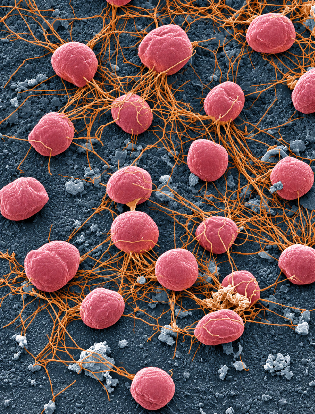
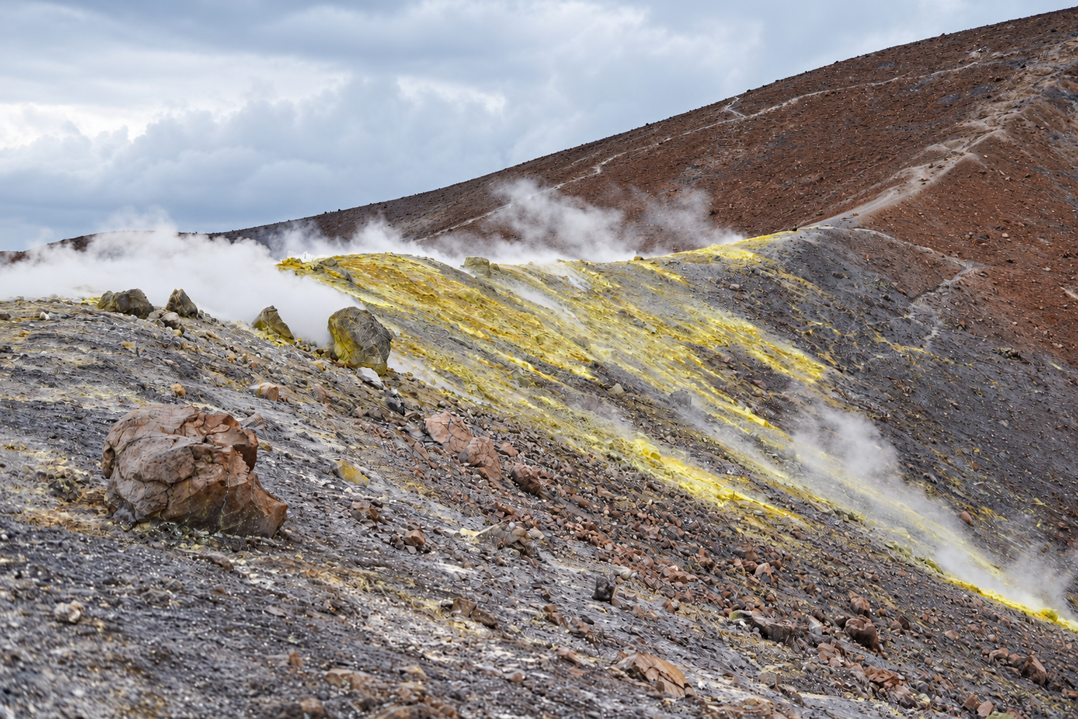
Researchers also studied a 653-base piece of its DNA that helped a small separate DNA molecule copy itself inside a specially prepared laboratory host. That gives us something interesting to compare when we study its chromosome. Will Ori Finder find a promising region here too?

Reference data — P. furiosus

Genome: NC_003413.1
Research: Farkas and colleagues, 2011

Pyrococcus horikoshii

Our third friend is P. horikoshii, found in the Okinawa Trough near Japan, at a depth of about 1,395 metres (4,580 feet). It grows best at around 98°C / 208°F, and its chromosome contains 1,738,505 bases.

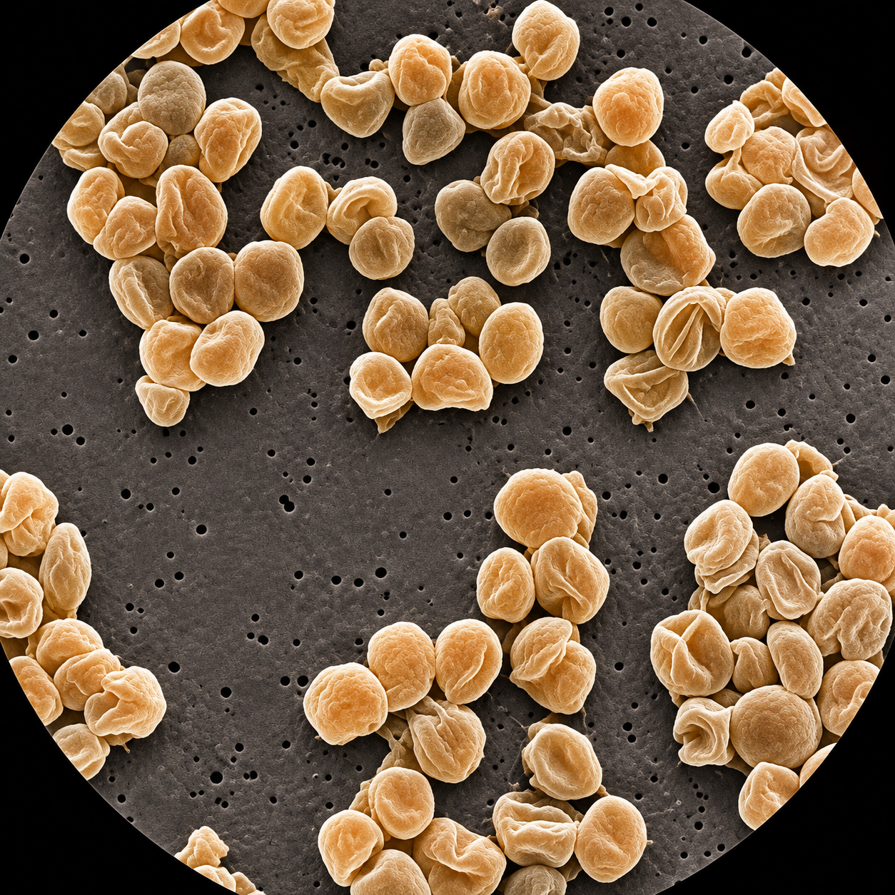
Researchers have also suggested a replication-origin region in P. horikoshii by comparing its DNA with related organisms. We’ll see what Ori Finder finds when we reach this genome.

Reference data — P. horikoshii

Genome: NC_000961.1
Origin comparison: historical DoriC annotation aORI10010007 (DoriC 12.0 database background)

A Project You Can Make Your Own

Ori Finder will be a small, independent Python project. In Part 2, we’ll create it with uv and download the real FASTA file. If you followed Genome Toolkit Part 4.2, you have already met uv, the modern Python project and package manager we use to create projects and manage their dependencies. We will use it here too. If it is new to you, you can review that Part or simply follow along: we will take the setup step by step in Ori Finder Part 2. We’ll keep the full P. abyssi chromosome and create a separate file with the known 799-letter region. Luckily, we already wrote the two algorithms we need to begin this investigation in Genome Toolkit. We’ll take simple versions of those pattern-counting functions and bring them into Ori Finder in ordinary Python, starting with a small example before moving to real DNA. Each new step will bring us closer to searching the whole chromosome.

We’ll also continue Genome Toolkit as a separate series. Ori Finder will focus on the biology and approachable Python; Genome Toolkit will show how to make the corresponding algorithms reusable and tested. You can follow either series or both. As a new biological question calls for another algorithm, we can try it in Ori Finder, check how it behaves with real data, and bring a reusable, tested version back into Genome Toolkit. The series can grow side by side: one follows the investigation, and the other develops the library that supports it. If you’re curious about where we’re taking Ori Finder and the larger Genome Toolkit project, you can read our quick Series Update.

Summary

With count_kmer(), we supply a DNA sequence and one exact pattern to count. With find_most_frequent_kmers(), we supply a sequence and a pattern length, and the function reports the most frequent patterns.

In the 799-letter P. abyssi region, all 787 of the 13-letter patterns we counted were different and appeared once. The paper gave us eight specific patterns to check, and five matched our sample once each.

Our next task is to search the complete chromosome without providing the already-known 799-base location. Ori Finder v1 will still use the research-informed 13-letter pattern family to rank candidate areas for further study, not identify exact initiation bases.

What’s Next?

In Ori Finder Part 2, we’ll create our Python project with uv, download the complete P. abyssi FASTA sequence, and save the known 799-letter region in a second FASTA file. Then we’ll write our first two functions, starting with a small DNA example before using our real sample.

We’ll take the DNA we’ve introduced here and start working with it ourselves. How do we pick out the right 799 letters from a chromosome of more than 1.7 million? And once we have them, what can our two functions tell us? We’ll find out together in Part 2.

Your Turn

Before we begin, here are two questions to think about: Why should we keep the complete chromosome FASTA when we create our smaller 799-letter file? And what would you like to count first when we have that DNA in Python? You don’t need to download anything or write code yet. We’ll start exploring these questions in the next Part.

We hope that exploring microbial genomes and the questions we can investigate with simple tools has been helpful to your bioinformatics and programming journey. If you found this Part useful for your journey into bioinformatics, biology and Python programming, and you’d like to help us keep creating free, open-source science education, you can support REBELSCIENCE. Your support helps us keep sharing what we learn and growing our community.

Until next time, rebelCoder, signing out.

Video version of this article: